
Created by Mark Grujic and Rian Dutch.

Recap
Welcome back to our series on drill chips! Here’s a quick summary of where we left off:
First, we went through the DOs & DON’Ts of capturing good quality chip photos.
Then we looked at how you can identify rock material within these photos, and create structured, informative datasets that map out the colour of rock chips.
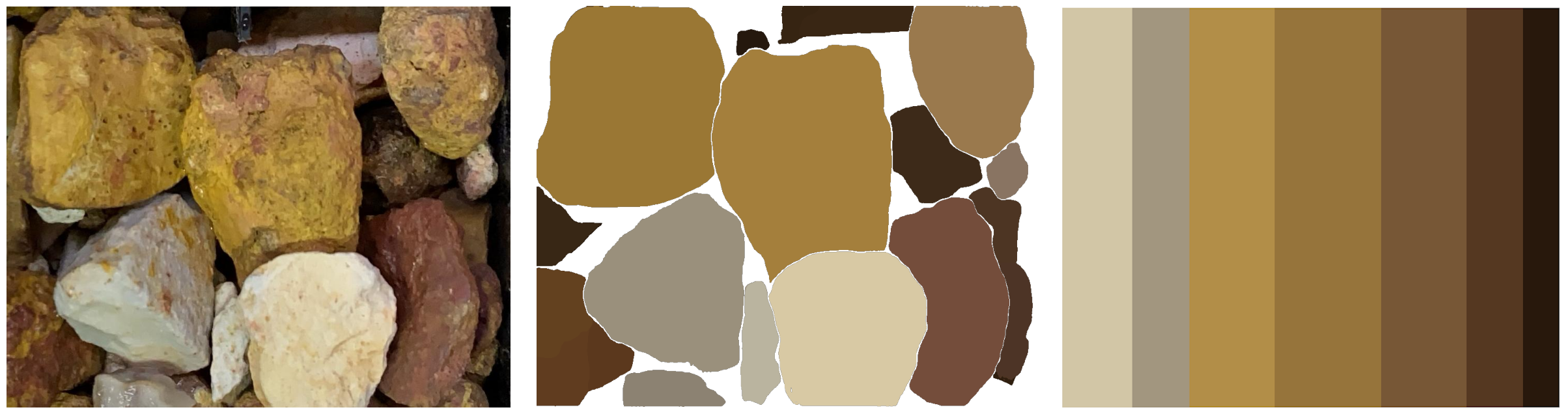
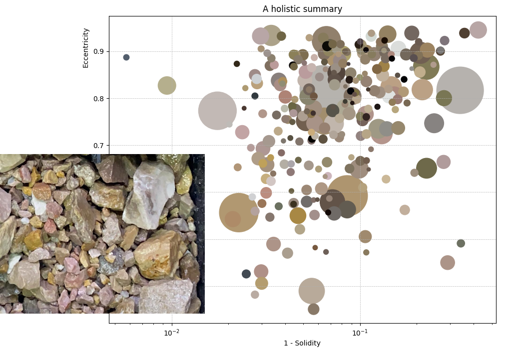
Then in the last update, we took it one step further to analyse the shape and colour of individual rock chips, resulting in quantified understanding of the variation in chip properties, in chip compartments and down hole.
Now – in this series finale – we will use additional deep learning techniques to further quantify rock chip character, and integrate everything we’ve done so far into a unified model.
Quantifying image data
Our goal is to represent our images as a series of numbers that characterise everything describable about the image. This encoding of visual information is an important step towards being able to answer questions like “where else looks like this?”.
We already partially encoded our images when we looked at extracting colour information in our colour blog. We took those colours and represented them as triplets of red, green and blue amplitude values as represented in the RGB colour model. This allowed us to look at similarly coloured images (below left), and the down hole variation in these colours (below right).
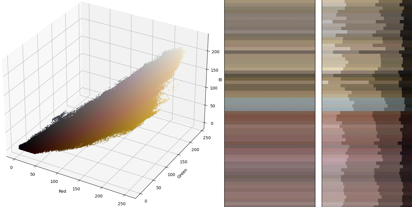
However, colour is only part of the geological equation. What if we want to encode our images to consider texture and other geological information as well? We can look at other techniques to extract features from images that better represent the whole image character.
One classical computer vision approach to extracting quantified information in images is to use texture features or Haralick features (Haralick, 1973). The intention of Haralick features is to provide a quantitative representation of the textural properties of an image, by analysing the spatial relationships between pixel intensities. A great visualisation of how Haralick texture features are generated is shown below, from Lofstedt et al. (2019, figure 1).
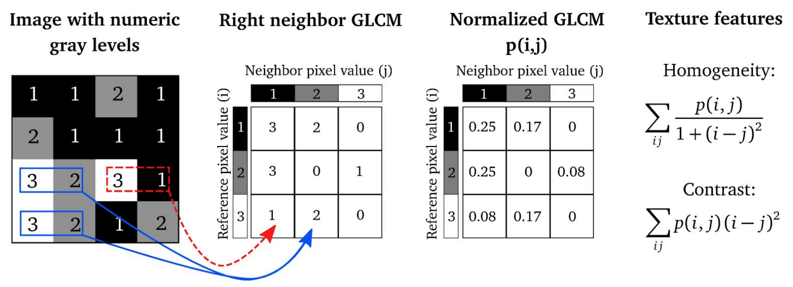
While efficient and perfectly suited to certain tasks, Haralick features aren’t capable of representing complex, high-level structure within images, as they operate on a grey-scale image and consider only individual pixels in relation to their surrounding pixels. Haralick features have also been shown (Monika et al., 2021) to be less effective than other methods at being able to perform downstream tasks on these encoded data.
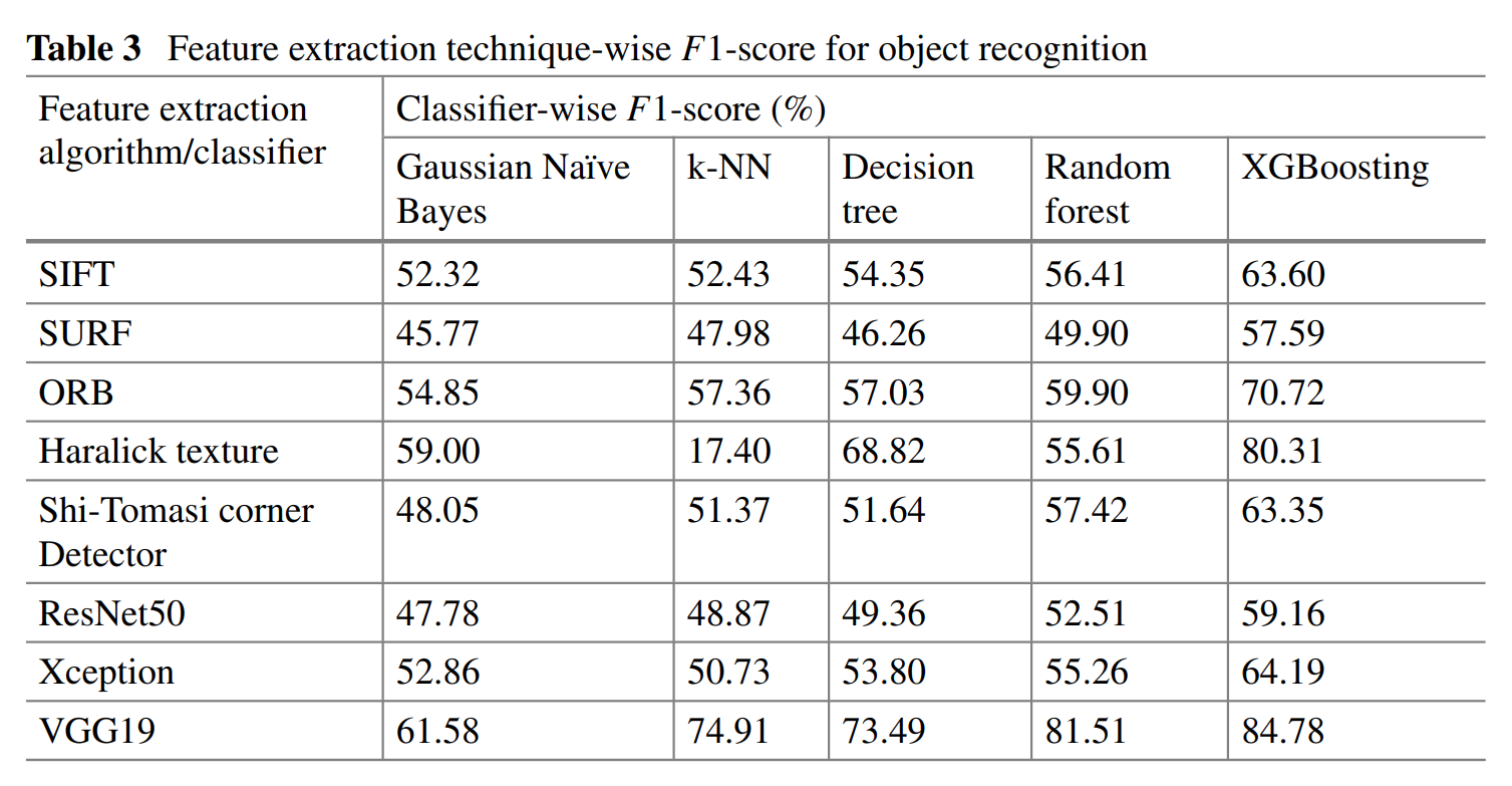
Table 3 from Monika et al. (2021), showing an example where Haralick texture features are less capable than other features at performing an object detection task on the Caltech-101 image dataset.
The specific task studied in Monika et al. (2021) was the ability to detect objects. We generally see these low-level, pixel-to-pixel features (like Haralick features) being outperformed by techniques that can capture both low and high-level information and retain an understanding of information hierarchy, particularly on complex tasks that need more than grey-scale features and representative colours.
Hierarchical feature extraction can be performed using algorithms such as Convolutional Neural Networks (CNN) or Vision Transformers (ViT). They work because they consist of multiple layers that progressively extract numeric features at different levels of abstraction. This captures both low-level features, like colours, edges and textures, and high-level semantic information, like contained object shapes, relative positions, and even categories or labels.
Let’s look at some of these more advanced (and more advantageous) algorithms in the context of drill chip images. The following is by no means an exhaustive explanation, and we encourage you to research or reach out to us if you have any questions.
CNNs – pretrained & fine-tuned
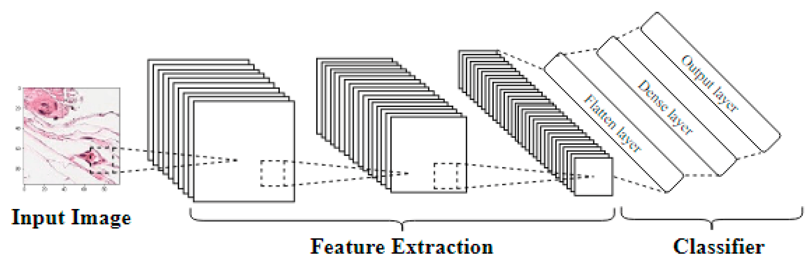
Pretrained CNNs are deep learning models that have been trained on large-scale image datasets, such as ImageNet (Deng et al., 2009). These networks consist of multiple layers of convolutional filters that can capture various visual patterns like edges, textures, and shapes, at different levels of abstraction, leading to hierarchical image features. Below, we see a schematic representation of how feature extraction relates to the convolutional layers of a CNN, from Kandel and Castelli (2020).
While not really an end-goal, the image features from these pretrained models provide a convenient starting point, allowing us to benefit from the learned features without having to train a network from scratch. Fortunately, we can fine-tune these pretrained models to make them better suited to a task at hand with our own rock chip image dataset. Image features extracted from this fine-tuned model are generally more beneficial for our purposes, however they require some target to model (e.g. a lithology log).
Self Supervised Learning
In the absence of a target to drive the fine-tuning process, it is feasible to perform Self Supervised Learning (SSL) on our chip image dataset, with the task of training a model to understand certain properties and relationships within the images themselves without the explicit need for labelled images (like the example of logged lithology). With sufficient images, SSL can learn dataset-specific representations, leading to more informative image features.
Vision Transformers
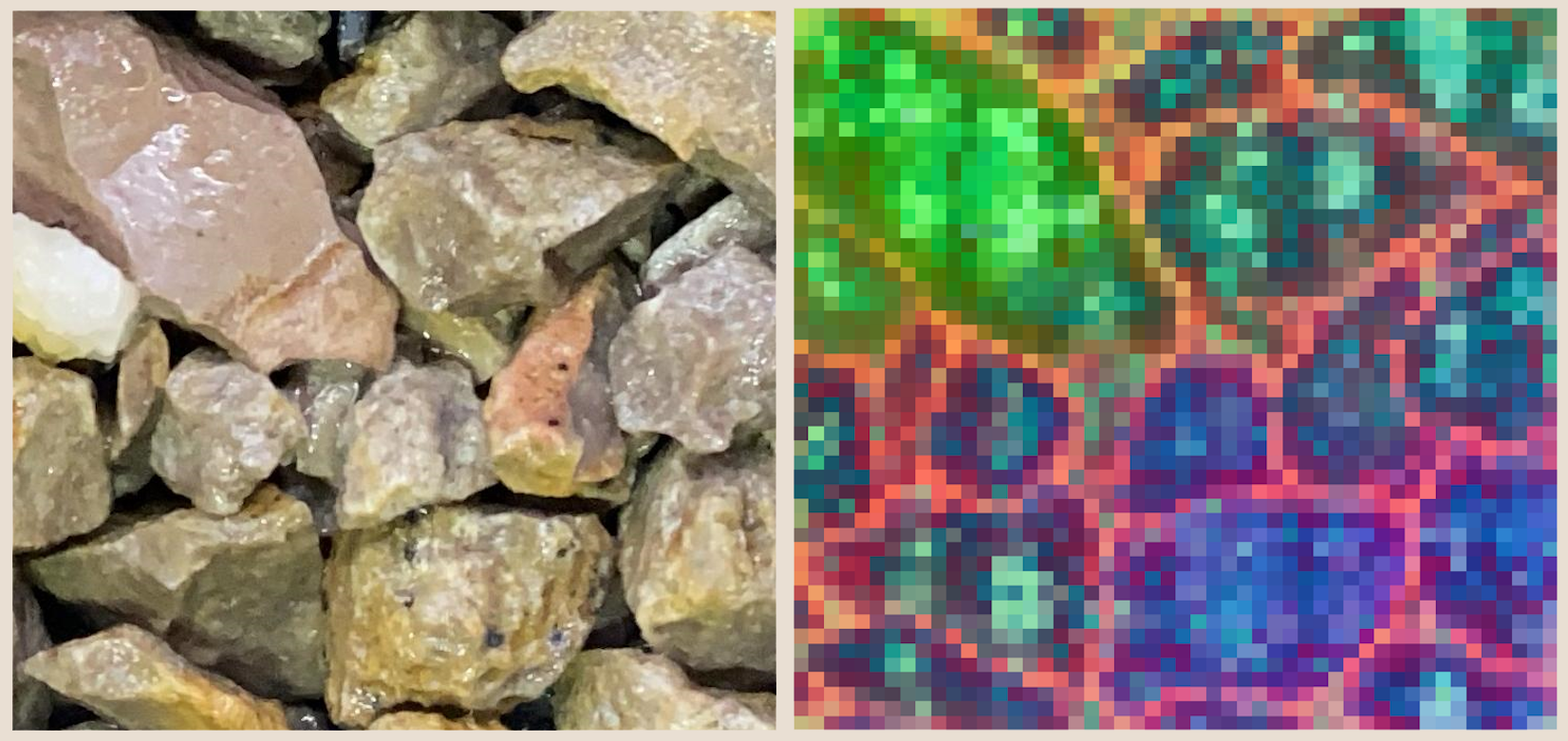
Somewhat the new kid on the block, Vision Transformers (ViT) are another kind of neural network where input images are divided into patches which are then processed. This approach can lead to a better understanding of the spatial relationship of geological features within an image, leading to spatially-aware image features.
Below, we see a dimension reduction of hundreds of image features per patch for a single chip compartment. The patches are the blocks seen on the right. Similar colours represent similar patches. More on this kind of thing soon.
Interpretation of features
Now that we have some quantified encoding of our image data, let’s explore some things that can help extract new or improved geoscientific understanding.
Image feature subspace
Hundreds (or even thousands!) of image features from hierarchical feature extraction processes can be unwieldy to deal with. Let’s reduce this high-dimension space to something more manageable. We could approach this in several ways, including:
- Changing the abstraction level that we select features from in our CNN
- Further processing of extracted features with a dimensionality reduction technique
Let’s expand on the last point, because there’s a lot of flexibility and possibility here. We’ll use the tried and tested UMAP algorithm (McInnes et al., 2019) to reduce our combined feature space, consisting of dominant colour, particle statistics, and image features (weighting each of these three inputs according to subject matter requirements). We reduce this combined image feature space to 2D. The claim is that even though this simplification to two dimensions does not capture the entirety of visual information in our chip photos – it’s a way of testing ideas in an easy-to-visualise coordinate system (noting that most further applications use the high-dimension data).
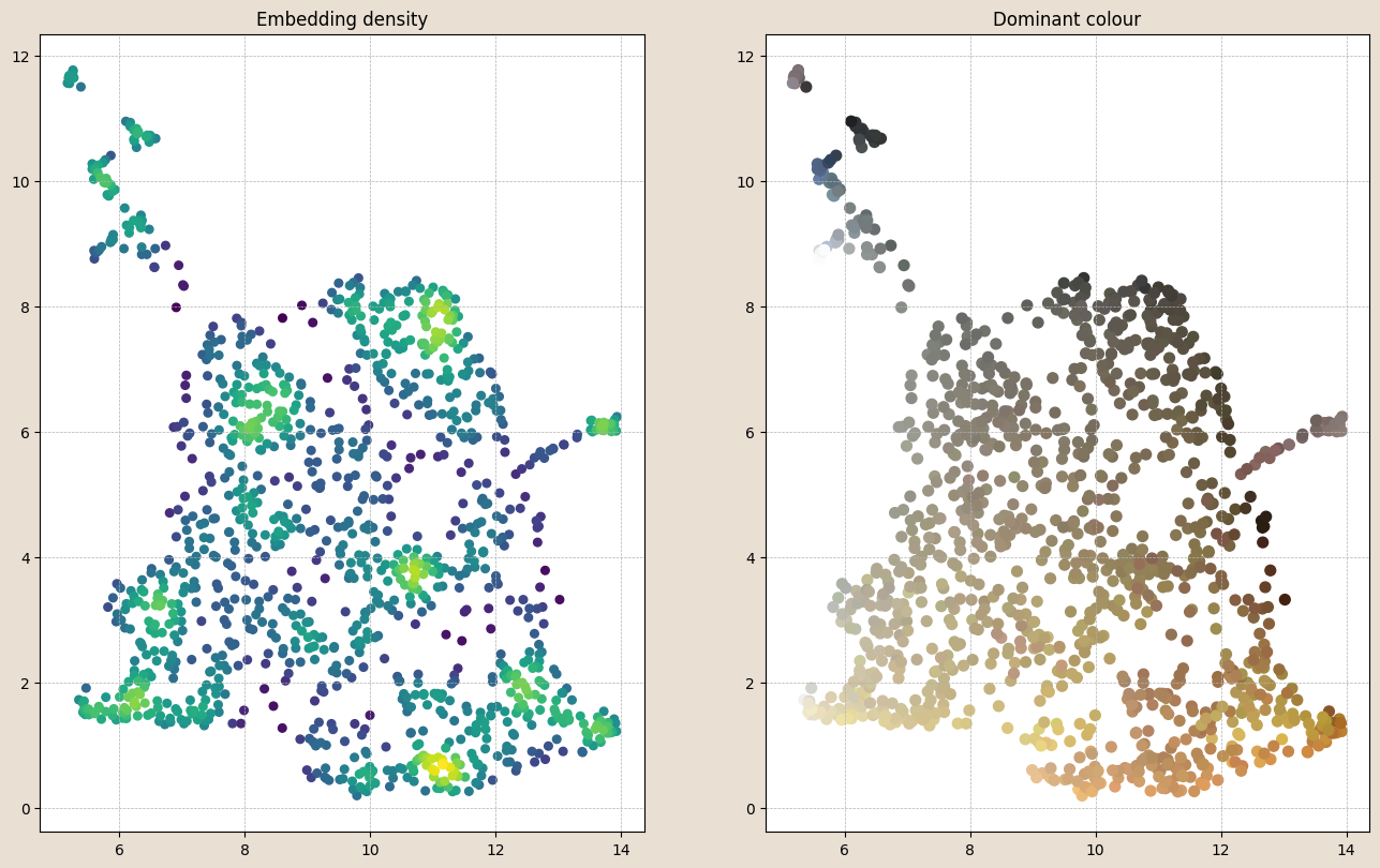
Below, each point represents a reduced-dimension coordinate for the individual chip compartments from our combined image feature space. We see that there are natural groups of images (left – coloured by density), as well as generally understandable transitions in dominant colour (right) across our feature subspace.
Visualising other components of our combined subspace (like mean particle size) can be performed in the same way. As a sanity check, we can also track a path through our subspace and look at the chip compartments at each step.
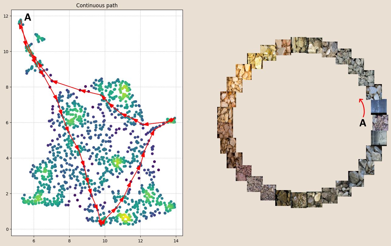
In this way, we can clearly assess the smooth and continuous nature of the rock chips at our project and start to answer questions like, “What looks similar to this?”, “how similar are these units?”, “What is the transition from A to B like?”, or the dreaded – “Did I log that properly?”. I’m sure your mind is running away with your own questions, given this kind of data representation.
The 2D coordinates shown are meaningful, but also just one way of representing similarity across a dataset of images. Below, we see the same combined image feature space forced into a grid, with an attempt to maintain global and local changes in feature subspace. The animation flicks between the dominant colour and the images themselves. It is apparent that with only colour, the full image character story is not told.

If you don’t like squares – you can also force the reprojection to a shape that might be more meaningful. For example if you know that your host rock was altered and took on two separate appearances, you could attempt to force your data to a Y-shape, modelling the branching different visual appearance. Or – you might just love your company and want to see its logo textured with transitional rock character 🤷.
![]()
Assigning a navigable coordinate system to images means that we can interactively explore images, assign labels to images, and log our data in this new context, as well as in the context of chip trays or core boxes and in 3D. At Datarock, we have internal software that lets you do this in an intuitive, interactive way, building up an understanding of the relationship between this subspace and the underlying data. Downstream applications include building a library of labelled image data and QCing existing categorical data such as geological logging.
![]()
Recolouring data
So far, we have generated some image subspace and embedded it in 2D, then looked at real data in that embedding (colour, images, statistics). We can also generate new datasets that make use of the combined image features in the subspace.
One example of a new dataset arises from the ability to generate a new colour for each chip compartment, derived from a dimension reduction of our combined dominant colour/chip statistics/image feature space. Here, we project the data to a spherical coordinate system, and then map colours to each coordinate using a Hue/Saturation/Lightness colour model. The spherical representation is shown on the left, and these colours are then plotted back to our 2D representation of the combined feature subspace.
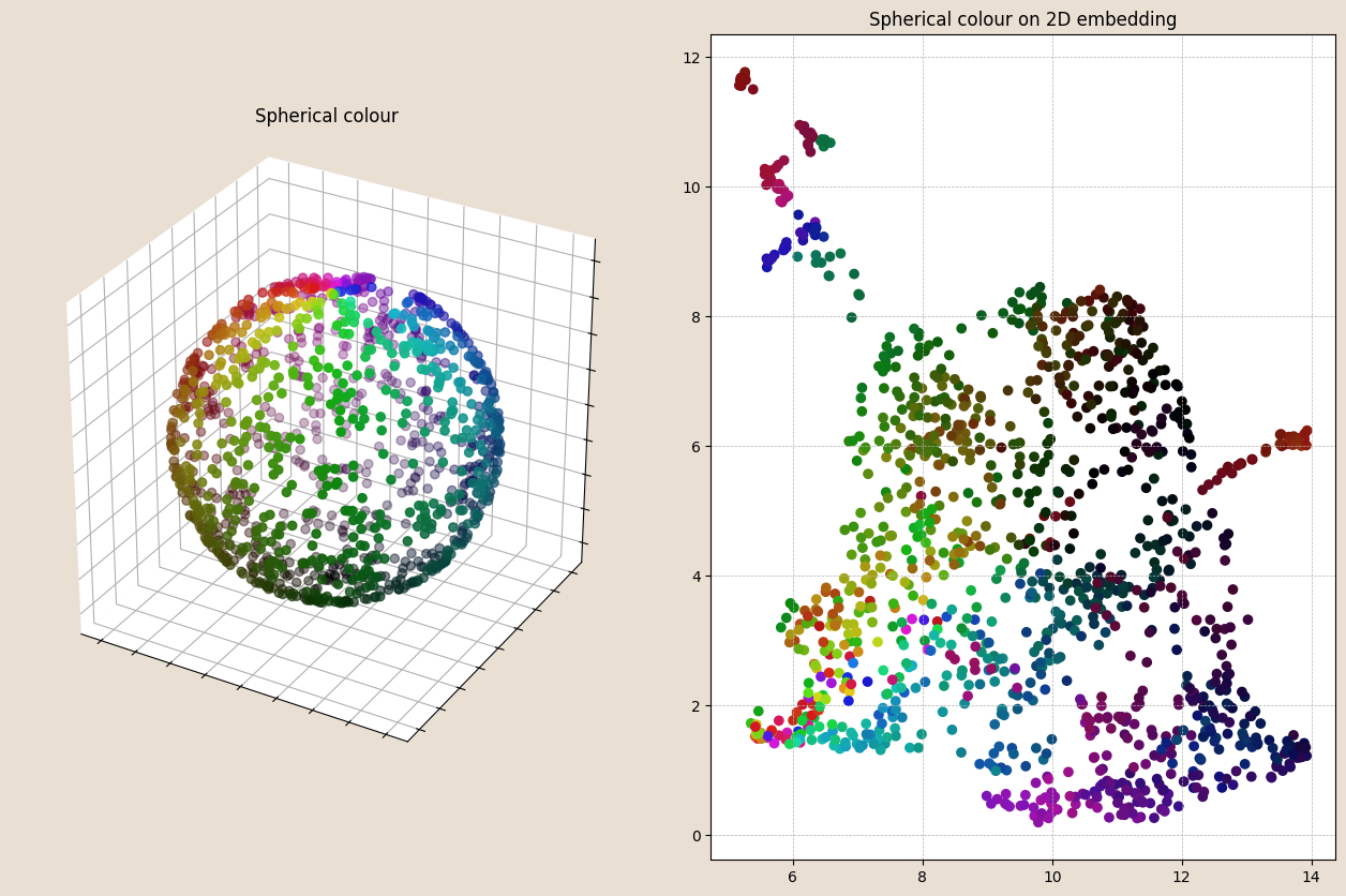
This makes it clear that while generally pretty consistent, there are sharp changes in colour in the 2D plot, suggesting that the 2D coordinates do not capture the variability captured by this recolouring exercise.
Clustering
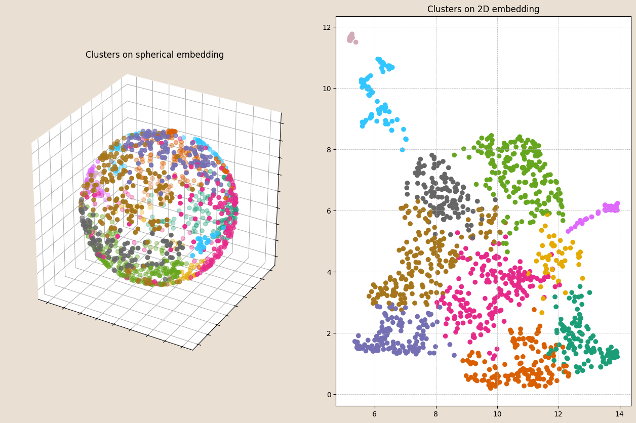
Another common new dataset that can be generated from this quantified image data is the grouping of similar images into clusters. The idea is that clusters are generally internally consistent, while being differentiated from other clusters. Below, we see the results of clustering applied to a network graph of our combined image features, presented on our reduced-dimension spherical and 2D cartesian coordinate systems.
Now we can do all sorts of things, like summarise things of interest within these clusters. For example, we can sample some number of images from each cluster.
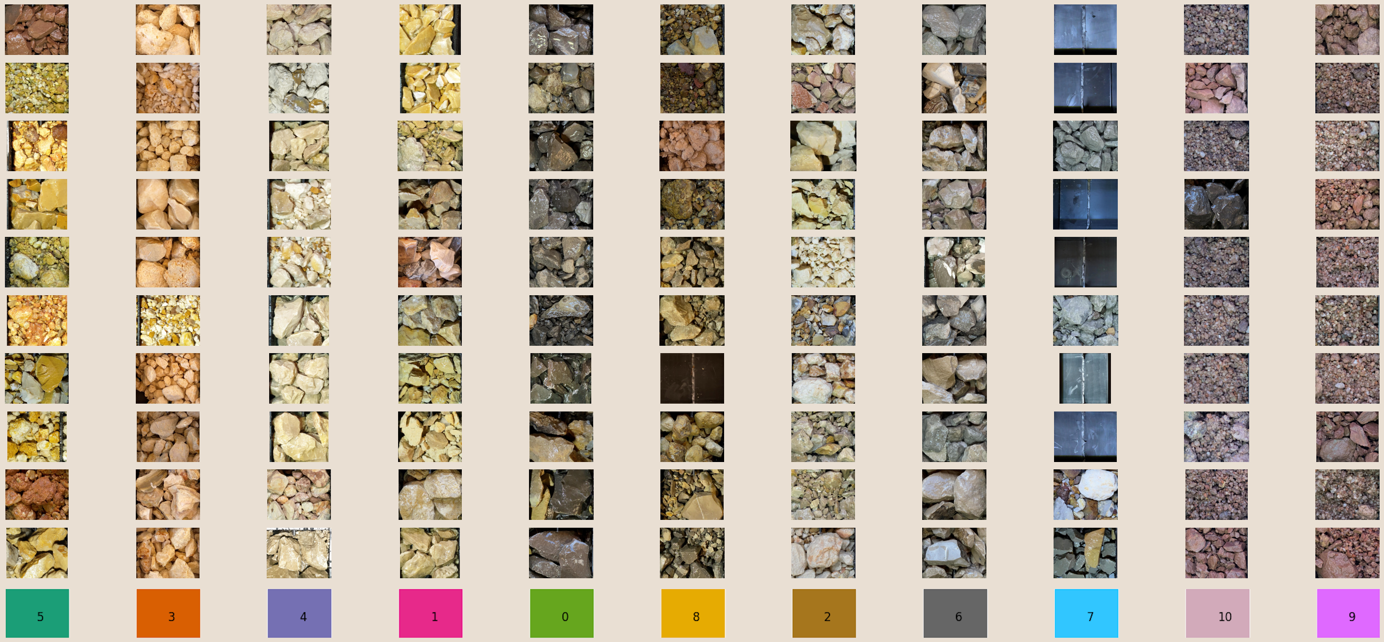
Here we see that there is general internal consistency, but there are some samples that don’t seem to fit with the rest. This is often an inevitable side effect of assigning clusters to a population where you force every data point to a cluster. We introduce hard boundaries on a continuous dataset (a topic worthy of another blog!). There are ways to minimise this, including only assigning clusters to very similar data/images and leaving uncertain data/images unassigned.
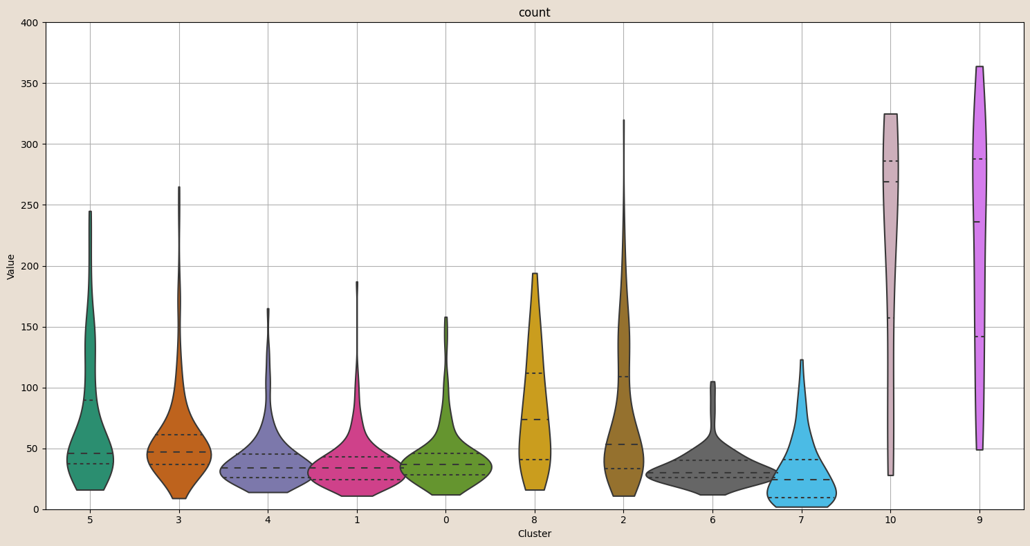
It’s also feasible to summarise statistics of importance within clusters, to determine if those statistics are characteristic of specific chip compartment groups. Below, we plot the median number of chips in each compartment, within clusters. We see clusters 9 and 10 have a significantly higher chip count than the rest of the population. This fits in well with what we see in the sample compartments above.
Integrating everything so far
Bringing everything from this blog series together, we can summarise our quantification of chip imagery into down hole logs. Here we see down hole changes in dominant and representative colours, key statistics including rock chip area distribution and count, our recoloured log that incorporates colour, chip segmentation statistics and hierarchical image features, and data-driven clusters.
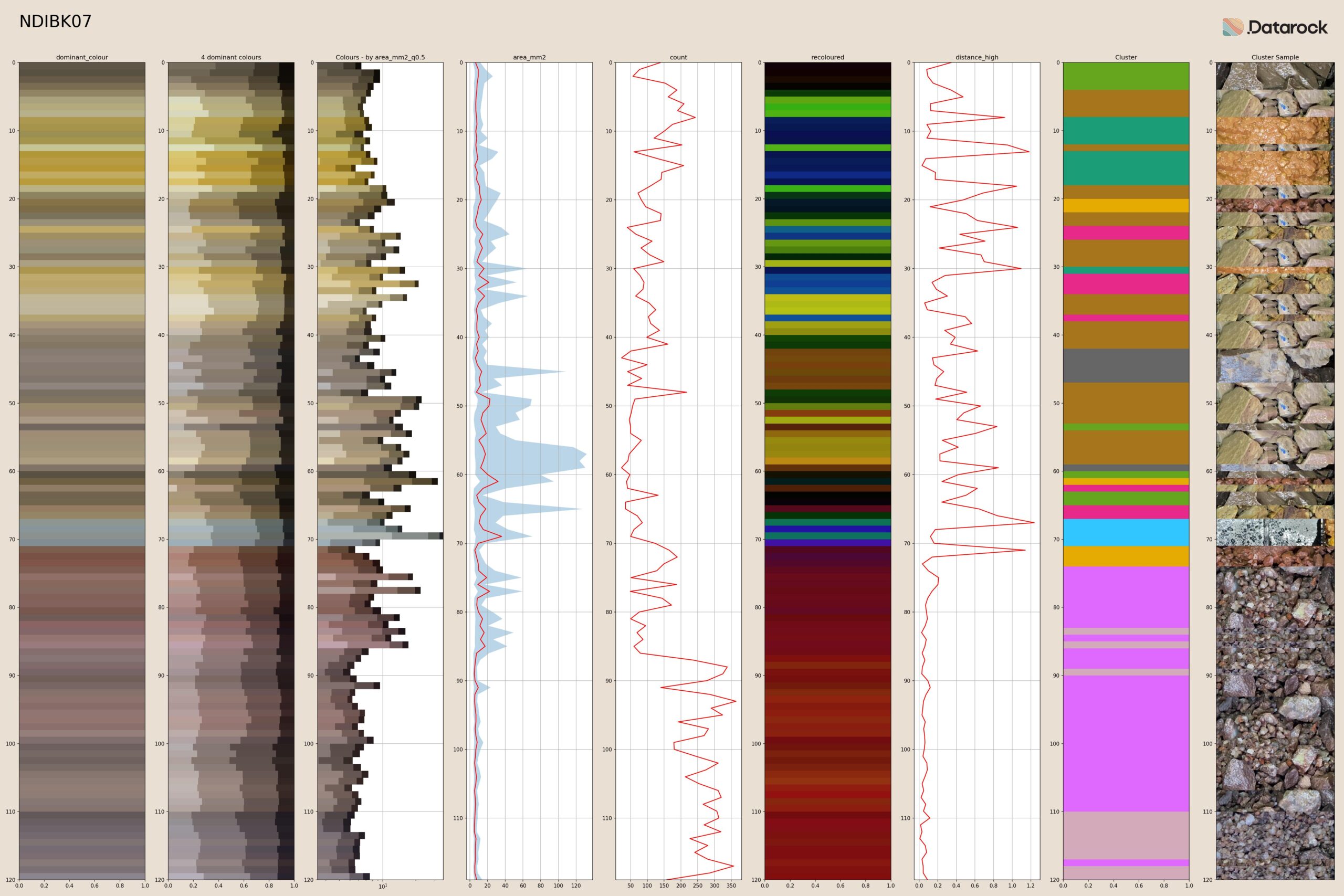
The third-last column in this plot was not discussed, but represents the down-hole change in combined quantified information – a proxy for geological changes. The last column is a fun attempt to create a textured strip-log, by using the most representative image from each cluster to texture the cluster log.
These quantified data are made available as readable text files, ready for incorporation into and 3D or mining software packages, to facilitate downstream decision-making processes.
Subject Matter Expertise
As we come to the end of this series, we wanted to address one key capability that has not been discussed. Geologists, geotechnical engineers and geoscientists of every discipline impart their own or their team’s knowledge into their workflows, based on available data and geological understanding.
Almost all of the processes described in this drill chip series benefit from incorporating SME knowledge. This could be as simple as changing the relative weighting of colour to hierarchical textures (e.g. logging lith, where it’s driven by colour). Stepping up a tier of involvement might see existing logged intervals used to train a custom prediction model, where the output is automated logging from photos. One step further could ask geoscientists to segment their own geological features of interest, like sulphide fragments in chip compartments, and then identify sulphide content across their project. Drill chip photos are far from the only informative data source available, so combining these technologies with other existing data (e.g. natural gamma) is a natural extension to any modelling exercise.
At Datarock, we believe that trained geoscientists and engineers have the most to gain from incorporating these and similar processes into their everyday tasks. That’s why – on top of all the wonderful data-driven work introduced in this series – we love to work with geoscientists to build and deploy models and capabilities that bake in their own bespoke knowledge and address specific needs. We believe that these technologies help geoscientists by making them even stronger in what they are already the best at; interpreting and making decisions.
Summary
Thanks for sticking with us for this entire blog series on quantifying drill chip photography. We hope you have a greater appreciation of the processes behind some of the things that we do and can be done with your geoscientific images.
At Datarock, we have built our business around doing this at scale, securely, and cost-effectively for our customers on their diamond drill core images. Our platform lets customers train custom models and infer the results across backlogs of historical data as well as in near-real-time on their ongoing drill programs.
All of the capability introduced in this chip photo blog series exists in Datarock for diamond drilling core photos, and we are rolling out the same capability for drill rock chip photos. If you would like to discuss, know more, or ask any questions that these articles might have inspired, please reach out to us.

“Essential geology tools in 2024” – Generated by StableDiffusionXL and “graphic design is my passion” guy.
References
Deng, J., Dong, W., Socher, R., Li, L. J., Li, K., Li, F. F., “ImageNet: A large-scale hierarchical image database,” 2009 IEEE Conference on Computer Vision and Pattern Recognition, pp. 248-255, 2009
Haralick, R. M., Shanmugam, K., Dinstein, I., “Textural Features for Image Classification,” IEEE Transactions on Systems, Man, and Cybernetics, vol. SMC-3, no. 6, pp. 610-621, Nov. 1973
Kandel, I., Castelli, M., “How Deeply to Fine-Tune a Convolutional Neural Network: A Case Study Using a Histopathology Dataset”, Appl. Sci. 2020, vol. 10, pp. 3359. 2020
Lofstedt, T., Brynolfsson, P., Asklund, T., Nyholm. T., Garpebring, A., “Gray-level invariant Haralick texture features”, PLoS ONE, 2019
McInnes, L., Healy, J., Saul, N., Grossberger, L., “UMAP: Uniform Manifold Approximation and Projection”, The Journal of Open Source Software, vol. 3, no. 29, pp. 861-, 2018
Monika, B., Munish, K., Manish, K., “Performance Comparison of Various Feature Extraction Methods for Object Recognition on Caltech-101 Image Dataset”, Select Proceedings of ICAAAIML 2020, 2020
