
Created by Mark Grujic and Rian Dutch.
Welcome back to our series on drill chips! Here’s a quick summary of where we left off:
First, we went through the DOs & DON’Ts of capturing good quality chip photos.
Then we looked at how you can identify rock material within these photos, and create structured, informative datasets that map out the colour of rock chips, and how they vary down hole. We looked at the representative colour of individual rock chips, and teased at doing more with each chip, to quantify as much information within our chip images as possible, and as promised – here we are!
Segmentation
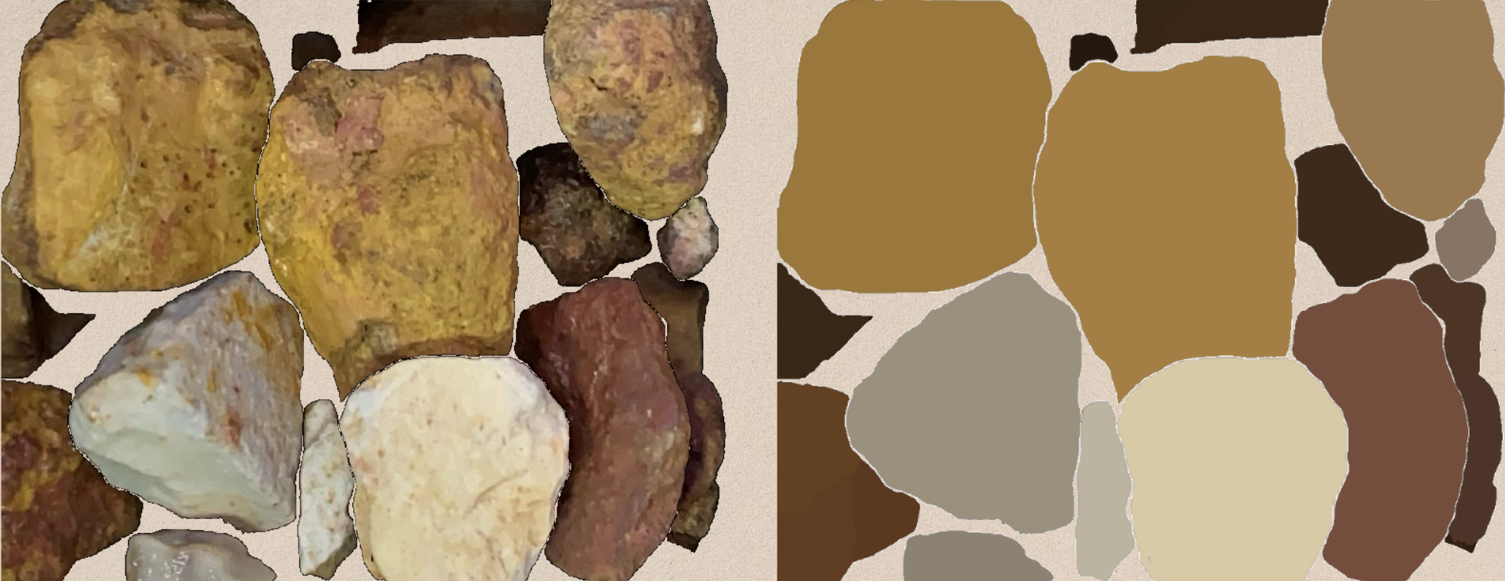
Taking a step back – let’s first review the process by which we can separate individual chips from each other, and other non-rock material in an image.
The figure below represents several common problems that we typically use computer vision to solve. The example uses veins as they appear in diamond drill core photos (a core Datarock product offering), along with some typical datasets that you can generate from each case. The same technologies are applicable to the rock chip study.
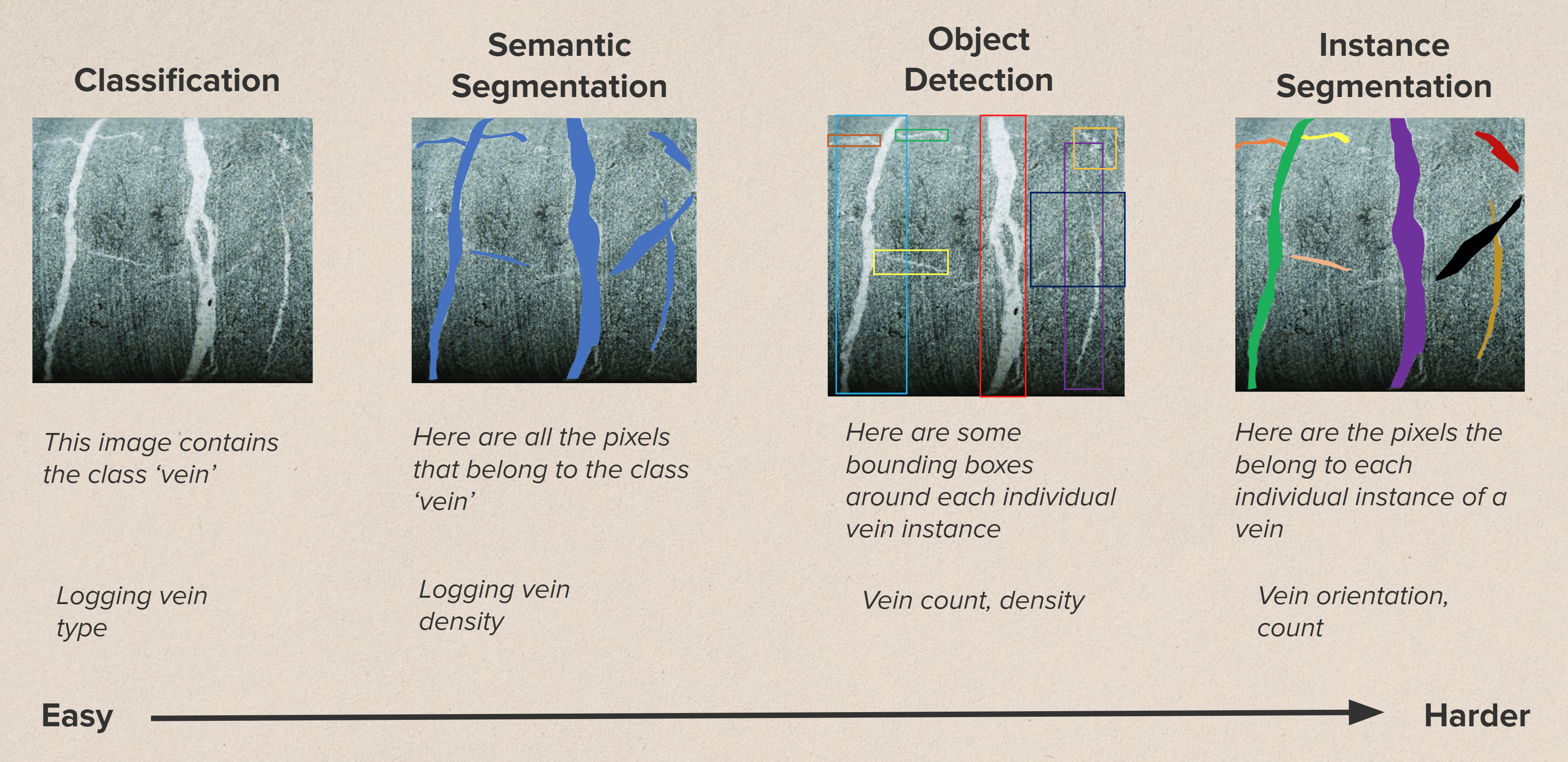
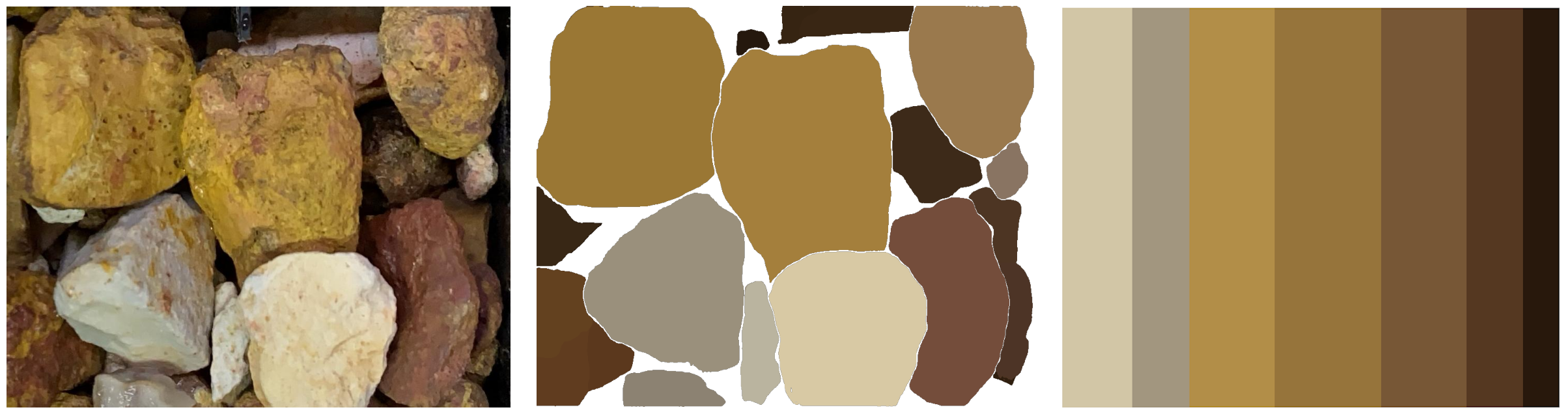
In the previous blog we used Semantic Segmentation to exclude non-rock material from the rock chip compartment colour analysis, and then Instance Segmentation to find the representative colour of each individual rock chip.
Chip Geometry
Given that our Instance Segmentation model has provided us with masks for each individual chip in all the compartments in our dataset, we can now consider the geometric properties of each chip, and attempt to produce geoscientific information.
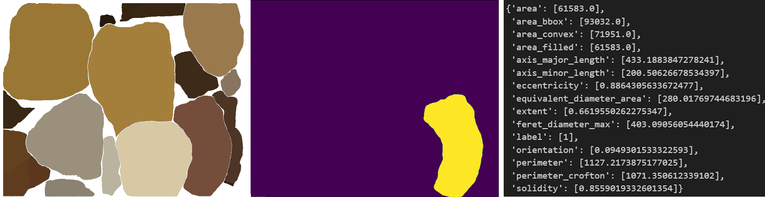
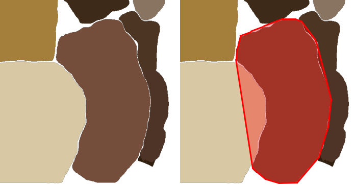
Fortunately for us, figuring out numbers that describe shapes is something that is well and truly established! For example, we can utilise the existing methodologies that Datarock uses for segmentation characterisation in our core photography products and services (e.g. vein orientation, fracture aperture, sulphide texture) to determine a number of parameters for each chip. Take this particular chip in the image below, and note some of the geometric properties that we can determine based on its mask:
There is a wide variety of different geometric properties that we could calculate for each chip, but let’s just focus on a few of them here that we think are important.
Area
An obvious choice – rock chip size distribution is a directly interpretable property and one of the primary drivers for demand for Datarock’s chip services. The area here is represented in pixels, so a length scale conversion should be applied. If you know something about the scale in your photos, with either a physical scale on the images, or by knowing the compartment width, area in pixels can be converted to area in millimetres squared or another real-world unit.
Eccentricity
This is a measure of how circular or elliptical a chip is. The closer the value to zero, the more circular the chip is. Values approaching 1 are very elliptical or very long. An example of eccentricity being geologically informative could be the interpretation of certain populations of chips that have preferentially broken along certain planes, resulting in one population with a higher eccentricity than another population.
Perimeter
Like area, knowing the perimeter of chips can provide useful size distribution information. Unlike area, this property does not scale with the square of the size unit, so variations might be more linear than area values. The most “efficient” area for a given perimeter is a circle, and we expect area and perimeter to scale similarly, however, unexpected variations could indicate chips with complex perimeters. Which brings us to…
Solidity
If you were to construct a convex hull around a chip mask (a polygon with no concavity between vertices), then calculate the area, it would always be greater than the area of the mask itself. The ratio of the chip area to that of its associated convex hull is known as its solidity, and ranges from 0 to 1. Values close to 1 suggest the perimeter of the chip is entirely convex (think regular geometric shapes), whereas small values suggest complexities in the chip boundary (rough, irregular). The example below has a solidity of 0.86.
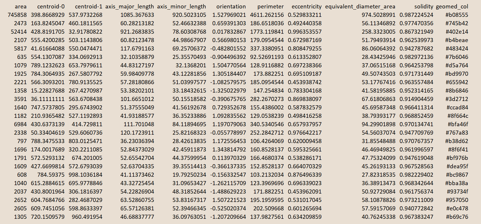
These statistics can be presented in a table, where each row represents a uniquely identified chip, and each column refers to specific geometric properties of the chip.
Some caveats
Caveats to the accuracy of these properties include the fact that we have a 2-dimensional representation of a 3D volume of rock chips, occlusion by other chips, lighting angles creating shadows, incorrectly cropped photos, and the accuracy of the chip segmentation model itself. These and more play a role in how certain you can be of the results of these geometric studies of individual chips and their summaries. However some assumptions can be made around these effects, and the way that the calculated properties change with depth can be just as informative as the absolute property values themselves.
An example of mitigating occlusion of chips by other chips would be assuming that the complex hull of a chip (see Solidity, above) is more representative of the chip’s true area than the visible mask. We can support this assumption with the understanding that rock chips fragment in relatively predictable ways that don’t result in crazy shapes that would result in very low Solidity. Another approach would be to identify all occluded chips and exclude them from the measurements.
Data scales
Geometric and colour properties of individual chips are all well and good, but as geoscientists, we are typically more interested in aggregating that information to more relevant scales.
Compartment scale
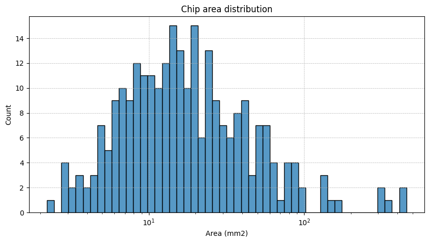
The first scale that we might consider interpreting is the information contained within each rock chip compartment. For each of our calculated properties on each chip, we can come up with statistical representations of their distributions within a compartment. This can give us a fairly straight forward understanding of things like chip size distribution:
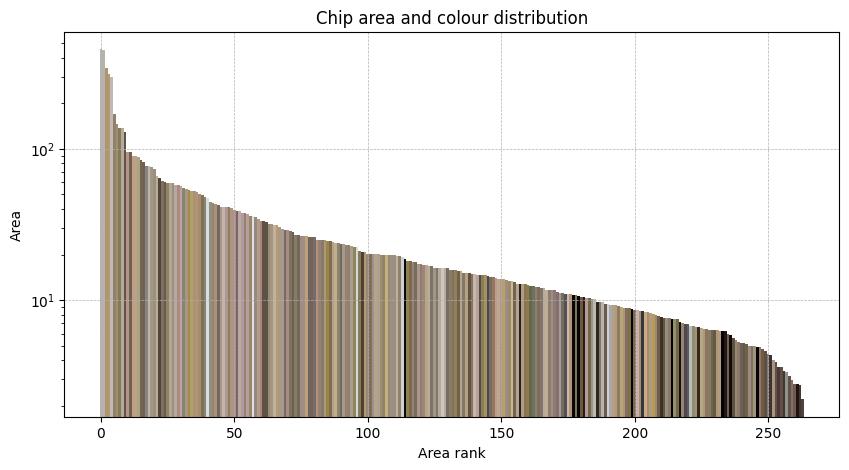
However, given that we have so much more information available to us for each chip, we can create some powerful datasets and visualisations to help interpret geology. For example, given that we already have the colour of each chip, we can do things like sort the chips by size, showing colour as another data property, and look for trends in size and colour:
We can also come up with our own project-specific set of plots that may help us answer the question we’re trying to solve. For example, the figure below shows eccentricity on the y-axis (how circular are the chips) against a measure of solidity on the x-axis (how complex is the perimeter). Each point represents a rock chip, with the size proportional to its area, and the colour being its dominant colour.
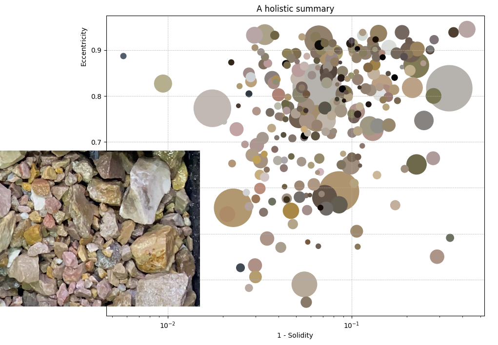
The ways you could combine and display properties of individual chips are almost limitless, so it’s important to think about what you are trying to solve, then build the right processes.
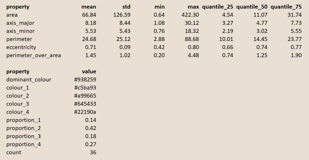
However, given that no single chip is representative of the compartment, we may also be inclined to statistically summarise the properties of all chips within a compartment, and represent the property distributions by things like their minimum, mean, maximum, median, standard deviation, etc. The tables below show some properties and their statistics within a single chip compartment, as well as the properties that cannot be summarised.
Drill hole scale
While the assessment on a chip-compartment scale can inform certain geoscientific or geotechnical decisions, we are often more interested in knowing the down hole character and variation of these quantified properties. As we see in the tables above, there are a lot of generated properties per compartment, and even more when we consider the statistical summaries! So, below is a subset of the available data, showing the median values in “area” to “perimeter over area” columns.
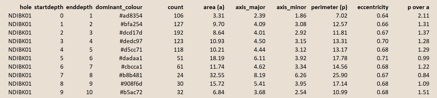
You might note that this is already in a neatly formatted table, thanks to good metadata tagging of the source photos, and the work described in the last blog in this series. Because of this, we can get to the final data visualisations in this blog – down hole logs showing how our calculated properties vary.
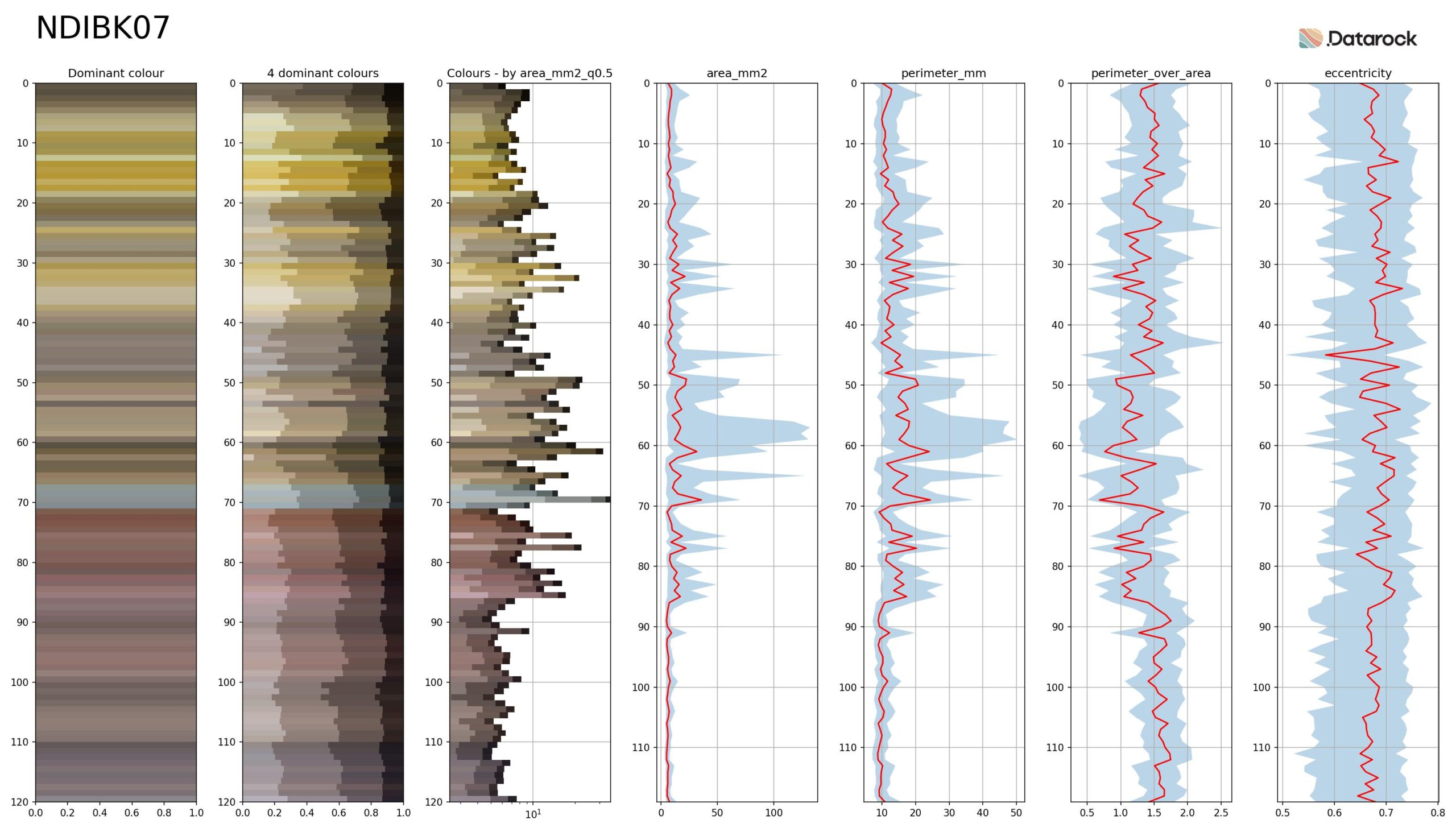
The first and second columns in these plots are the same as we saw in our earlier blog on colour. The third column is the same as the second, except the bars have been scaled by the median chip area in each compartment, resulting in a product greater than the sum of its parts. The rest of the columns are downhole logs of the variation in some key properties, showing the median in red, and the 0.25 and 0.75 quantiles shaded in blue.
These tables can (should!) be brought into your own modelling software for integration with other datasets.
Wrap up
We’ve seen how to ensure that your chip photos are good and properly tagged with metadata. Then we looked at how to extract and use colour information. In this update, we’ve addressed quantified chip geometry and how to incorporate it with earlier work, to then extract geological information. These powerful datasets generated from an often overlooked data source can become a valuable part of your geological and geotechnical workflows.
As chip photo collection processes improve over time, and as we are all being asked to do more with our datasets, we see Datarock Chip (the productionisation of these capabilities), working hand in hand with our drill core imagery products and services on your projects.
The story doesn’t end here! The next blog in this series on drill chips will introduce how we incorporate deep-learning based computer vision technologies into this process of quantifying visual information in rock chips, before tying everything presented to date into a single interpretive dataset. Stay tuned!
![]()
