
Created by Mark Grujic and Rian Dutch.
TL;DR: Chip tray photos are one of the most underused datasets in exploration. This blog explains how geologists can extract quantitative colour information from chip imagery using computer vision and colour models. Starting with simple cropping or automated compartment detection, the analysis identifies representative colours for entire compartments, individual chips, or chip-only pixels. These colour profiles reveal meaningful geological variation downhole and lay the groundwork for more advanced insights such as lithology discrimination, sulphide estimation, and automated chip logging. This is the first step in transforming chip photography from a visual reference into a structured, quantitative dataset for modern geological interpretation.
In our guidelines about how to take an analytics ready chip tray photograph, we emphasise that, as is the case in all good data acquisition processes, the first step is to capture the best possible dataset to analyse.
In this blog, we will begin the process of analysing and extracting useful quantitative datasets from good quality chip tray photographs, on the way to be able to develop meaningful, actionable, insights from this type of ubiquitous and underutilised dataset.
The first step on this road is to extract and analyse the most obvious parameter we as geologists see and use when logging chip trays – colour. Geologists rely heavily on the interpretation of colours observed in rocks, particularly in core and chip samples, as they provide valuable insights into various geological aspects. Colour plays a crucial role in representing geologically meaningful characteristics such as lithology, alteration, and mineralogy. By closely examining the colours present in a rock sample, geologists can discern important information about its composition, and better understand the sample in relation to surrounding geology.
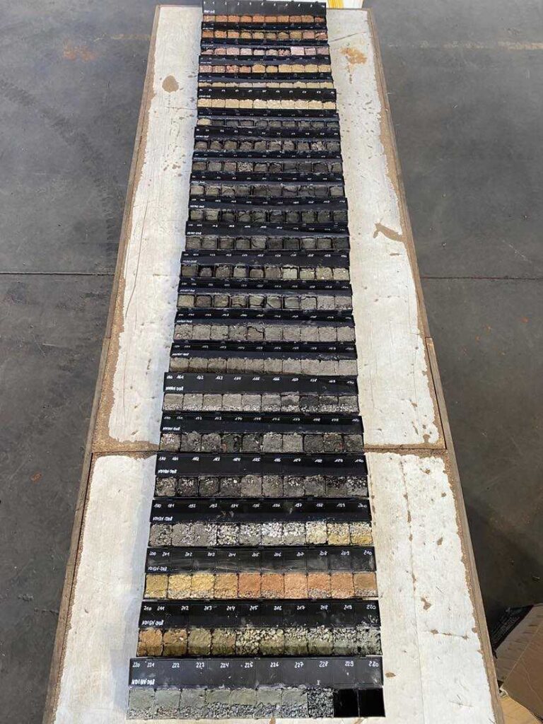
An example of the obvious colour variation seen in an example Coiled Tube drill hole as the drilling samples various lithologies down hole. Image from the Geological Survey of South Australia.
Photos to data
Arguably the most challenging, is taking an unstructured dataset like a chip tray photo and turning it into something that we can then use to extract information on a compartment by compartment basis. There are several ways this can be done. The Datarock Platform, which extracts and analyses quantitative data from core imagery, uses a series of computer vision models to transform a raw photo into an analytics ready core segment. Similarly, this approach can be taken using chip tray images. Given the huge variation in available chip tray images (see our previous blog for examples), this is an interesting problem and will be discussed further in an upcoming blog in this series.
The simpler way to approach this problem, which only works where you have consistently presented photographs, is to simply use a geometric template to consistently crop individual compartments from an image. It is important to also capture the spatial information along with each compartment image, so that all further analysis is depth constrained.

Automated compartment extraction based on a regular geometric template. Image from Geoscience Australia.
Quantifying colour
What are meaningful questions to ask when attempting to study colour and its variation within a geoscientific image dataset, such as chip photos? Every project will have different objectives and asks of their data. In this blog, we attempt to answer some general questions that are more or less independent of the geological context, to establish a baseline from which a trained professional can build on.
Assuming that we have our cropped images of rock chip material within compartments, with minimal background and otherwise unwanted content, we can study the colour of our data as represented by several different contexts, and ask some key questions:
Within each compartment representing a depth interval in a drill hole, what colour or colours describe:
- Everything in the compartment?
- Everything in the compartment that is a rock chip?
- Each individual rock chip?
How do these colours vary down hole and in 3D space?
A colour primer
To identify a colour that best represents an image, we need to understand that colour can be numerically represented in many, many ways (https://en.wikipedia.org/wiki/Color_model), called colour models. When an image, stored as a jpg or png or other file format, is loaded into a computer, the colour of each pixel can be numerically represented by passing saved information to any of these colour models.
One of the most intuitive colour models to think about is the RGB model (https://en.wikipedia.org/wiki/RGB_color_model), where the red, green and blue primary colours of light are added together to form a distinct colour. Using this model, the colour of each pixel in our loaded image is therefore defined by an RGB triplet (r,g,b) of numerical information.
Since this colour model uses three components, we can geometrically represent colours by assigning each component to an axis in cartesian space, resulting in a colour cube that defines all possible colours available to the colour model.

Each pixel within our image can be represented as a point in this r/g/b cartesian space.


What colours describe everything in the compartment?
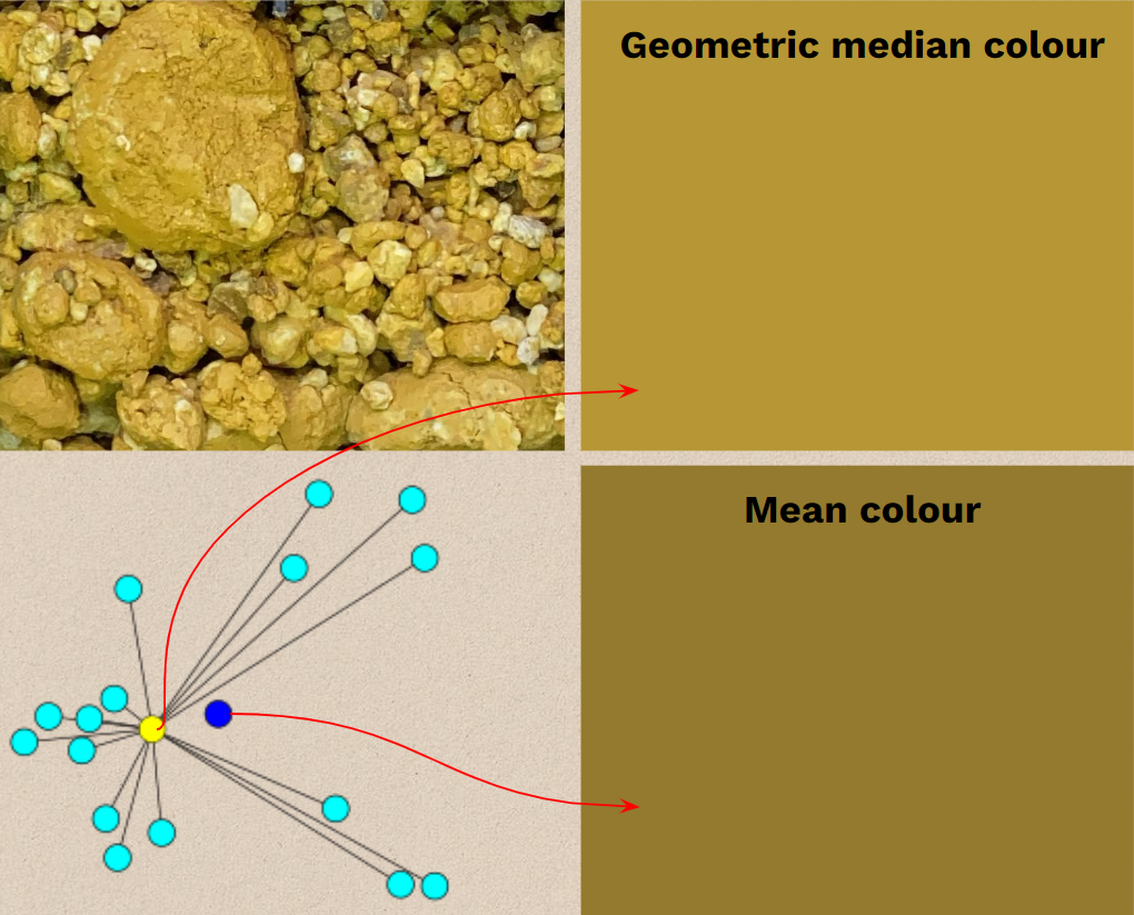
Given that we have a model of all of the colours in our chip compartment image (r,g,b triplets), we can very simply calculate the mean of each of our red, green and blue values. The resulting mean colour could be considered representative of the image.
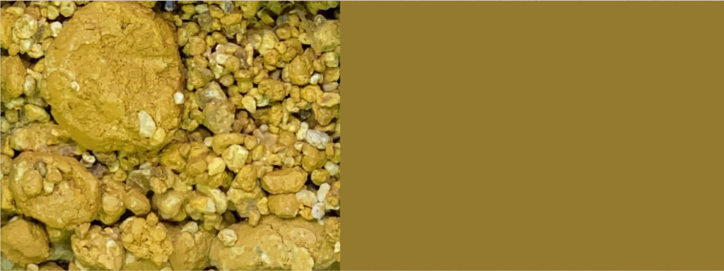
However, imagine a compartment with blue rock chips and red rock chips. The mean colour would be purple, which is not at all representative of our rock material! In certain statistical scenarios, the median value of a distribution is often considered more representative than the mean. We can extend the concept of Median to higher dimensional space, to find the geometric median of the r,g,b cartesian values in our image, ensuring that the resulting colour does indeed exist and is as representative of the image as possible.
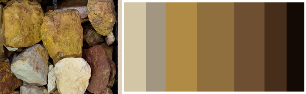
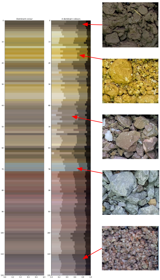
We can further extend this assessment of representative colours to capture multiple colours, and the proportion of the image that each represents. For example, below we see a rock chip compartment along with the 7 colours that best describe the contained material. The widths of each colour signifies the proportion of the compartment that it represents.
Using this approach, we can now begin to build a complete colour profile for each compartment down hole. Below is an example of this, showing a log of the top 4 representative colours in each compartment downhole.
However, you may notice that there are some colour artefacts creeping into this analysis. For example in the below animation, you can see that the black colour actually represents the dark shadows in the chip image, and are not representative of an actual piece of rock. To get around this, and open up the opportunity to extract even more information from each compartment, we can use another computer vision model to segment each individual grain.
What colours describe rock chip material?
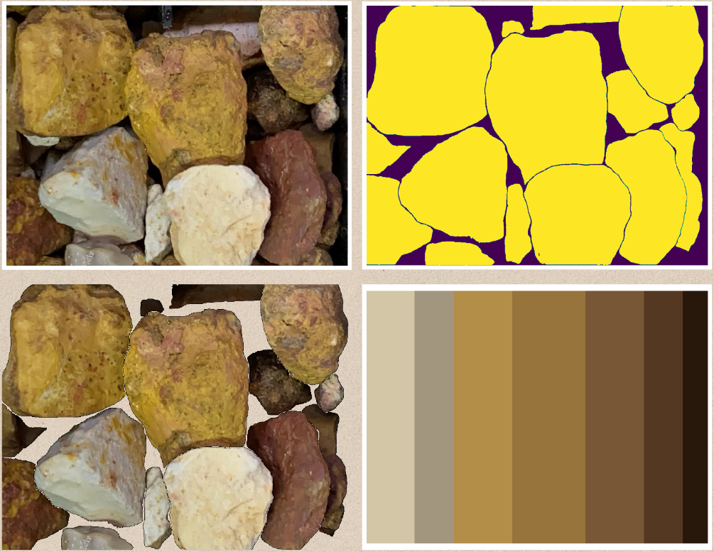
Just like it’s possible to use a segmentation model to isolate the chip trays and compartments, we can also use one to isolate chips within an image. In the below image we go from the original chip image top left. Then using a semantic segmentation model we can identify chips from the image and create a binary mask (top right). Using this we can then extract just the pixels representing chips from the image (bottom left) and finally, undertake a similar colour extraction process to that described above to capture the representative colours for only the chips within the image (bottom right).
What colours describe each rock chip?
Taking this one step further, instead of a binary mask that distinguishes rock chip material from background material, we can isolate each individual rock chip and extract the single most representative colour using the described processes. Below, we see the rock chips from the instance segmentation model on the left, and the geometric median colour for each distinct chip on the right.
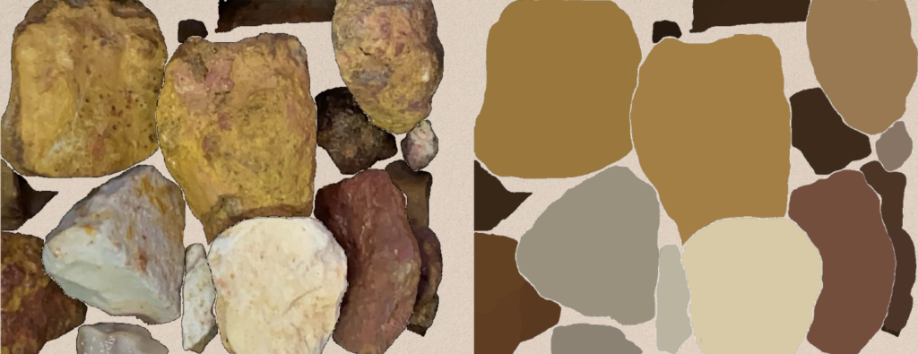
The power of this more detailed, individual chip segmentation opens up further avenues for extracting data about each chip, such as information about size and morphology, which we will go into more detail on in the next blog in our rock chip series.
Summary
In this blog, we’ve tried to walk through some of the potential types of information, focused around colour, which can be automatically extracted from chip tray photography. In some exploration settings, this information could go a long way to automating your chip tray logging and providing important information about where in the system you are.
The processes described in this blog are very general and applicable to all sorts of rock chip photos (as well as many other geoscientific image datasets!). However, there is so much potential to extract more guided colour information from your specific photos. For example, if your chips consisted of mixed lithologies such as granitic chips mixed with mafic dykes, we could begin to identify and classify the lithologies in each compartment just on an analysis of the colours. Or, if your chips contained sulphides, it would be possible to count the sulphide pixels and generate some proportion statistics, just from an analysis of the colours.
As powerful as an appropriate analysis of rock colour is, it is also just the entree to the feast of quantified data that you can automatically extract from the humble chip tray photo.
In the next blog in this series, we’ll show how we extract morphological information from the rock within your images, to really start to build a quantitative dataset to aid in your geological interpretations. Stay tuned!
