Created by Mahsa Paknezhad and Jack Maughan

In remote sensing-related geological modelling projects, a common challenge arises when geological signatures are affected by human-made infrastructure artefacts such as roads, dams, power lines, mines and buildings. These artefacts cause distinct variations in surface reflectance or artificial geophysical anomalies, creating misleading results in machine learning applications. Masking these artefacts could mitigate the problem; but it risks omitting valuable geological information. To address this issue, we are developing an alternative approach to masking by using stable diffusion to learn from surrounding regions and inpaint to approximate the real data beneath the artefacts. Although this approach is still a work in progress, the current results are compelling.

Remote Sensing

In spectral remote sensing, the physical characteristics of an area are quantified by measuring its reflected and emitted radiation from a distance, typically via satellite or aircraft. The unique reflection and absorption properties of various materials allow us to identify the materials from which the light is reflected. This information is invaluable for mapping surface geology and detecting compositional changes of the Earth’s surface.

In this project, we used Sentinel-2 data, captured by the Sentinel-2 satellites equipped with a multispectral imaging instrument known as MSI. Our project focused on the Northern Flinders Ranges in South Australia, specifically over the Beverley and Four Mile roll-front uranium deposits. We selected this region mainly due to its compositional variation in surface infrastructure, including calcrete roads, operating plants, and mud pits.

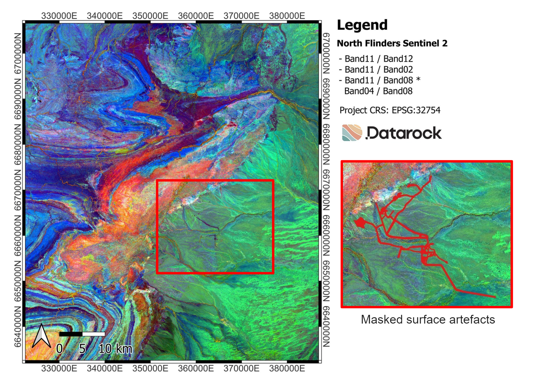
Figure 1: Figure shows an RGB false colour composite of Sentinel-2 data at North Flinders ranges in South Australia. Most surface infrastructure artefacts were identified and masked. The masked regions are shown in red. 

Sentinel-2 data captures 13 spectral bands ranging from visible to near-infrared to shortwave infrared wavelengths. Excluding band 10, which is used for atmospheric corrections, we have imagery consisting of 12 spectral bands. Since these bands have different spatial resolutions, we upsampled all bands to a uniform 10-metre resolution. 

To better visualise these 12 bands, we generated an RGB false colour composite image using bands 2, 4, 8A, 11 and 12 (Figure 1). The red channel represents the hydroxyl index, calculated as the ratio of band 11 to band 12. The green channel represents the iron oxide index, calculated as the ratio of band 11 to band 2. The blue channel represents the vegetation index, calculated as the ratio of band 11 to band 8A multiplied by the ratio of band 4 to band 8A. It is important to note that the RGB composite image is used only for visualisation purposes; the modelling is conducted using all 12 bands.

We identified and masked most surface infrastructure artefacts in the Sentinel-2 imagery of the North Flinders Ranges. Figure 1 shows these masked regions. Next, we will explain the inpainting method used in this project.

Inpainting Method

Inpainting has been frequently used in computer vision to reconstruct missing or undesirable parts of an image. Traditionally, inpainting involved utilising neighbouring pixels and interpolating their values. However, with advancements in vision transformers and generative AI, diffusion models have emerged as the preferred method for inpainting. Figure 2 shows a typical application of inpainting in photo editing tools. 

Figure 2: Figure shows a common application of inpainting, which is also available in new smartphones. Photo credit: https://www.perfectcorp.com/

Diffusion models in computer vision represent a class of generative models that can produce high-quality images. Inpainting and text-to-image generation are two typical applications of diffusion models. In this project, we deployed the Latent Diffusion Model (LDM), shown in Figure 3. The training of LDM is done in two phases. In the first phase, a convolutional neural network named UNet is trained to reconstruct masked regions within input images. In the second phase, the UNet undergoes fine-tuning using a diffusion-based denoising objective.

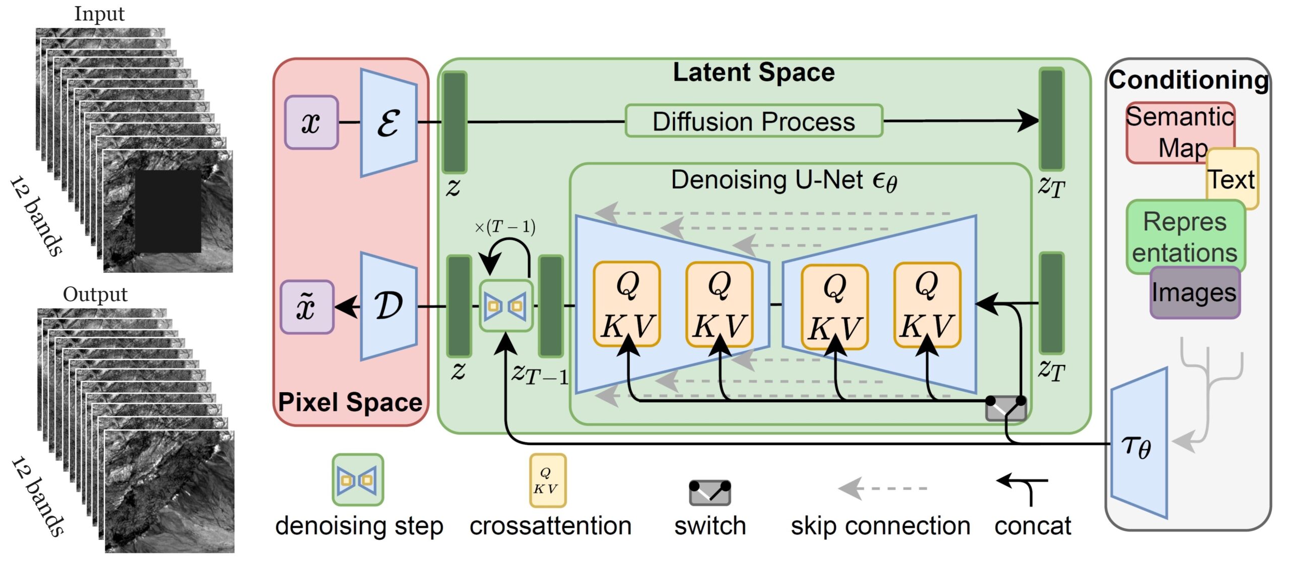
Figure 3: Figure shows the architecture of the Latent Diffusion Model (LDM) used for inpainting. The architecture was adapted to accommodate images with arbitrary numbers of bands.

We faced several challenges when adapting LDM for remote sensing imagery data. Firstly, existing LDMs are developed for RGB images, whereas our imagery consists of 12 spectral bands. Additionally, the typical input size for LDM is 512 by 512 pixels, while our imagery is substantially larger, approximately 6,500 by 7,500 pixels. To address these challenges, we re-implemented multiple components within the LDM architecture to accommodate images with an arbitrary number of bands and initialised the new LDM model with the weights of a pretrained LDM model. We then cropped small tiles from the Sentinel-2 imagery with no surface infrastructure artefacts and fine-tuned the LDM on those tiles. During training, random box masks were generated to simulate areas with artefacts.

Once the model is trained, we use it to inpaint tiles with identified surface infrastructure artefacts. Figure 4 shows three examples of tiles with surface infrastructure artefacts. The mask specifying the surface infrastructure artefacts in each tile is shown in the second column.  We convert these masks into box masks following the model’s training protocol and apply them to the tiles. The masked tiles are then fed to the LDM, which replaces the masked regions with the generated output. The replacement process involves a gradual transition from the original imagery to the inpainted imagery, guided by the smudged mask generated from the original mask. The final inpainted images are shown in the last column.

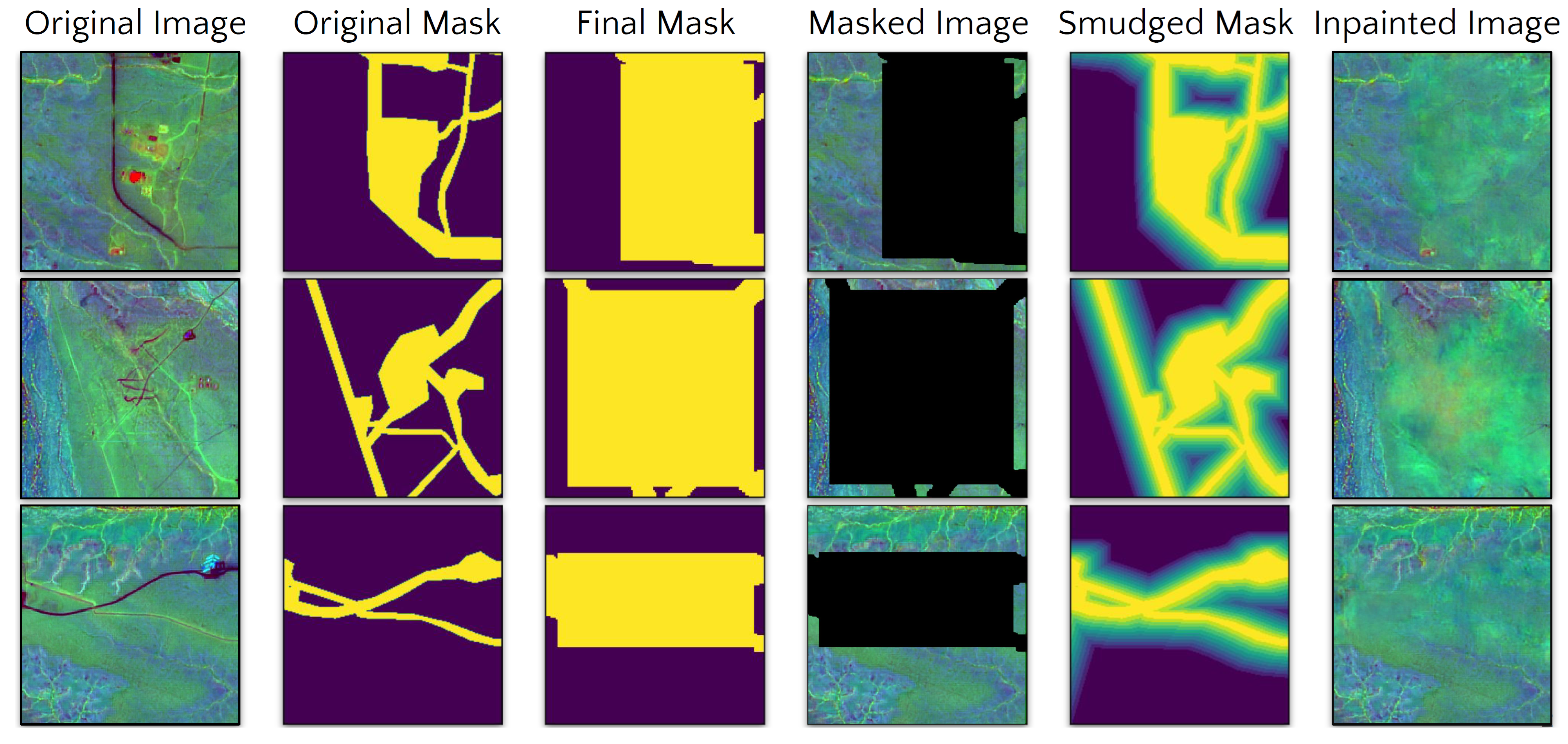
Figure 4: Figure shows how the trained LDM model is used to inpaint tiles with surface infrastructure artefacts.  

In total, 52 overlapping tiles, each measuring 2 by 2 km, were cropped from the region with surface infrastructure artefacts (Figure 5). The tiles were inpainted as previously described and merged together using feathering which ensures a smooth transition between adjacent tiles. Finally, the merged inpainted tiles were integrated with the non-corrupted regions of the imagery. Figure 6 shows the original imagery with surface infrastructure artefacts in North Flinders Ranges from Sentinel-2 data, the identified and masked surface infrastructure artefacts, and the imagery after inpainting.

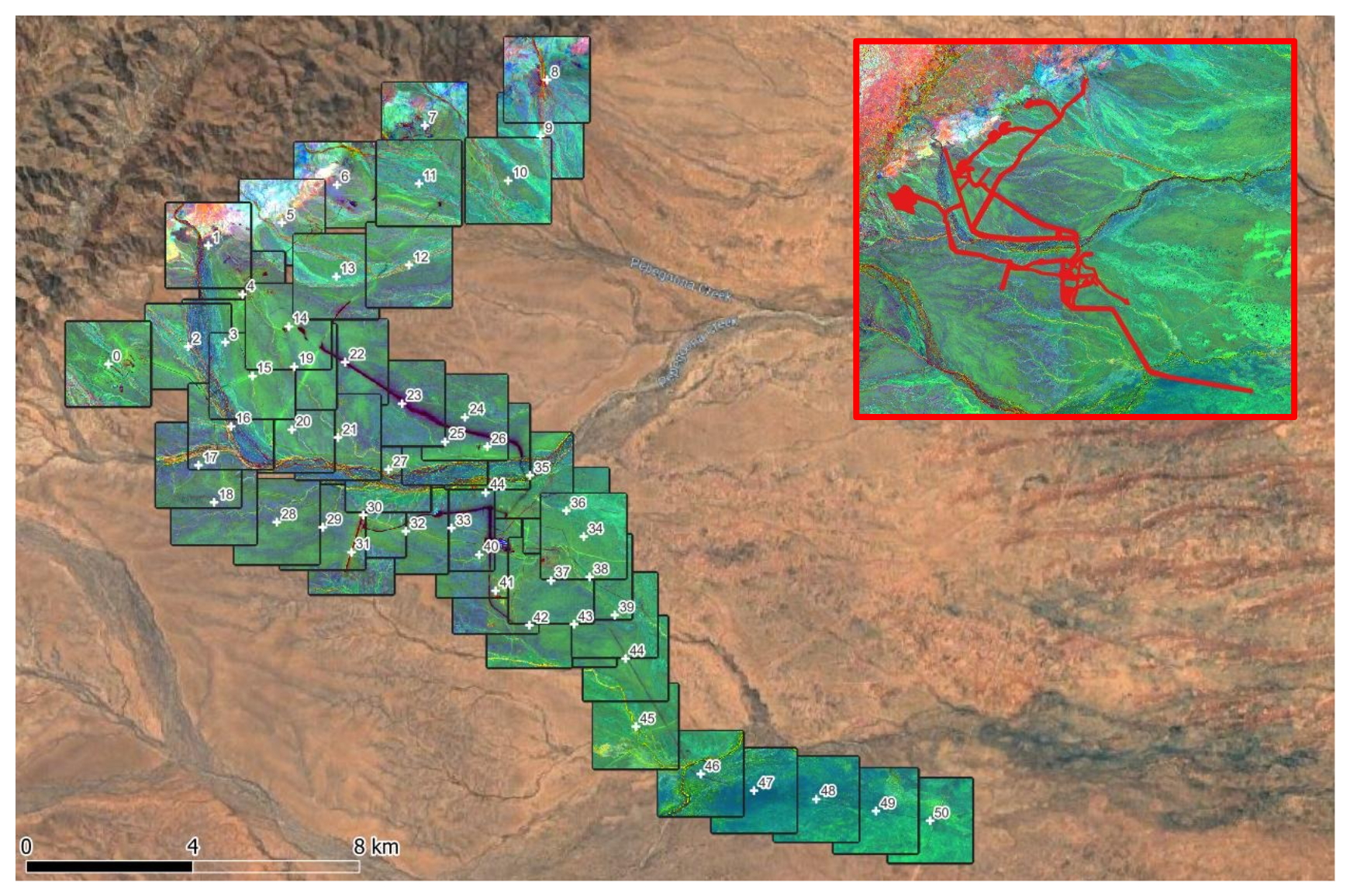
Figure 5: In total, 52 overlapping tiles, each of size 2x2km, were cropped from the region with surface infrastructure artefacts.

Figure 6: Figure shows the original Sentinel-2 imagery of the North Flinders Ranges with surface infrastructure artefact, the corresponding masked imagery, and the imagery after inpainting.

Potential Improvements

There is definitely room for improvement, as the model has not yet managed to provide detailed and structurally continuous inpainting. One potential improvement involves utilising the same style of masks observed in the input dataset, rather than using box masks during training. This could enhance the model’s focus on the corrupted regions but may require longer training times. Additionally, training the UNet in LDM with attention modules could maintain better structural continuity in the imagery data, addressing the discontinuity that arises in the inpainted regions. This would necessitate training the model from scratch, requiring substantially longer training time compared to the 16 GPU days we spent on fine-tuning. Another improvement could involve using a better tile merging algorithm to mitigate the occasional appearance of edge effects in certain parts of the imagery. 

To illustrate the issue regarding structural discontinuity more clearly, we selected a region of Sentinel-2 data that does not contain any structural artefacts (Figure 7 (Left)). We then generated and masked a fake road in this region (Figure 7 (Middle)). After applying inpainting to the masked region, we compared the output of the inpainting model (Figure 7 (Right)) with the original data (Figure 7 (Left)). As can be seen, certain regions lack desirable structural continuity. We hope that the aforementioned improvements will mitigate this problem.

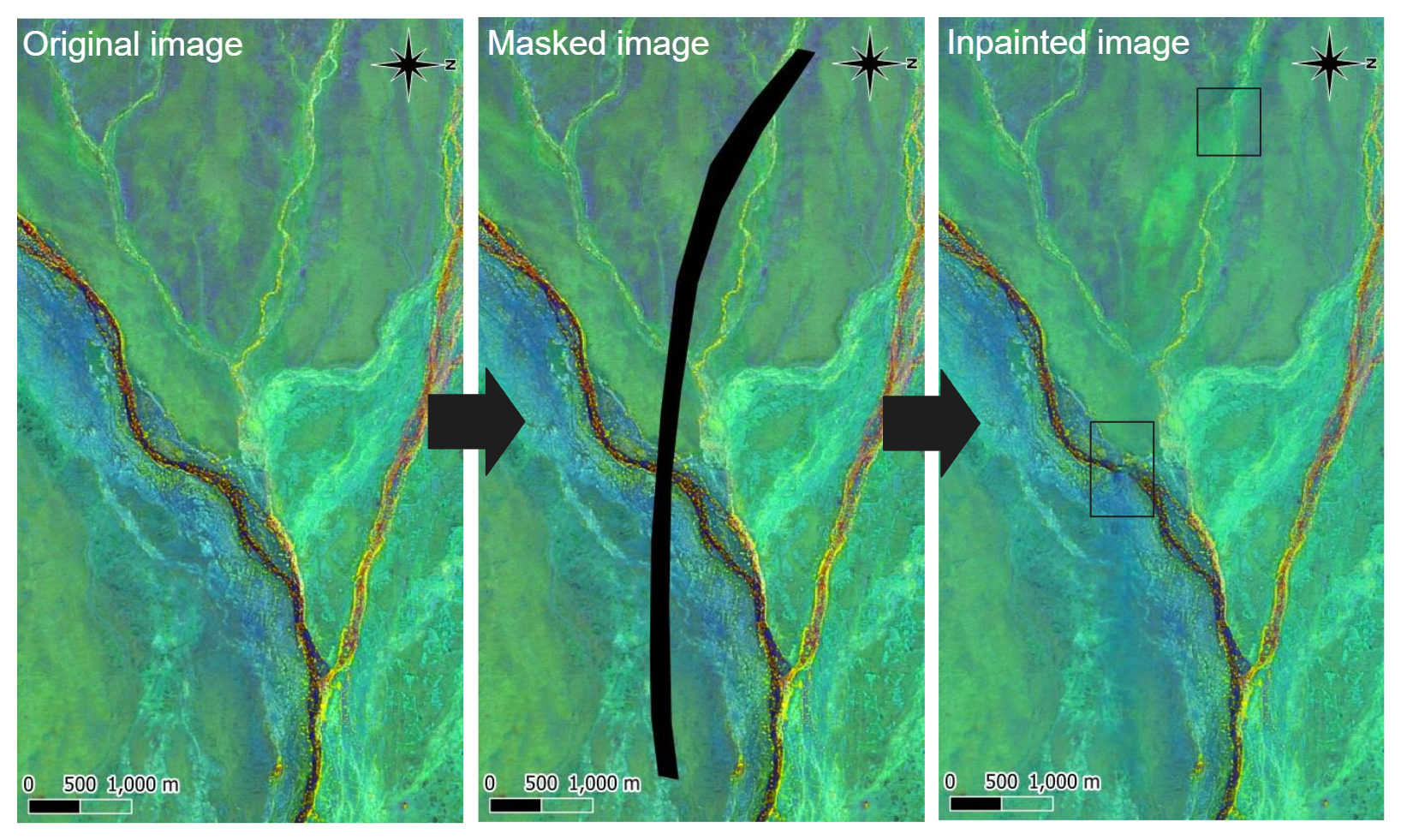
Figure 7: In an experiment, we applied the trained inpainting model to a region without surface infrastructure artefacts by generating and masking a fake road in that area. This enabled a direct comparison between the inpainted output and the original data. The bounding boxes highlight regions where the structural continuity in the inpainting model’s output is weaker than expected.

Conclusion

We believe that our method for multispectral satellite inpainting will add great value to current geology modelling workflows as it matures. In contrast to conventional methods of interpolation, LDMs utilise complex spatial context from learned real surface data to provide a more robust approach to inpainting. Moreover, this blog post only addresses the inpainting of one specific type of remote sensing imagery: Sentinel-2 data. In reality, however, this methodology can be applied to various forms of gridded spatial data such as hyperspectral and potential field geophysics, enabling removal of unwanted artefacts. Exciting times lie ahead for spatial image processing!