“I thought this model was supposed to work really well. Why has it started spitting out things that don’t make sense?”

Machine learning models can bring huge benefits in exploration and mining, but sometimes, it can seem like models that once worked well have started to go off the rails. This post is about why that can happen.

Even well-trained models aren’t immune to the challenges of working with evolving data. Over time, their predictions can drift away from reality. This drift occurs when the data going into the model changes, or when the model’s understanding of that data is no longer relevant. A model trained on early drilling results, for example, might miss important changes in mineralization patterns as a project evolves. In this post, we’ll break down two fundamental types of drift – data drift and concept drift – and explore how they show up in the mining industry.

What is drift?

If you start reading the literature on drift, you’ll probably get confused quickly. There are so many terms: data drift, concept drift, covariate shift, virtual drift, sampling shift, feature change, prior-probability drift, global drift, target shift, and many more (see table 1 in Bayram et al, 2022).

You’ll also notice that these are sometimes defined using mathematical notations like P(X), P(y|X), P(X, y).

Despite the confusing terminology, there are just two core types of drift to understand:

• Data drift occurs when the input data changes – the model sees something it’s never encountered before
• Concept drift occurs when the relationship between inputs and outcomes changes – even if the data looks the same, it means something different now

The mathematical notations allow us to define these concepts precisely (and concisely). What we call “data drift”, others sometimes call “covariate shift” – but both can be defined with a notation like P(X). Let’s come back to the notation later, and start with building an intuitive understanding of the two types of drift.

Data drift: When the model encounters something new

Let’s say you’ve trained a machine learning model to classify lithologies based on photos of drillcore. During the initial program, you use historical photos from a range of different camera setups and lighting. The model performs well and is put into production.

Since this exercise was so useful, you decide to improve your core photos following Datarock’s advice. You start taking photos inside using a controlled light source and with a higher-resolution camera (Fig 1).

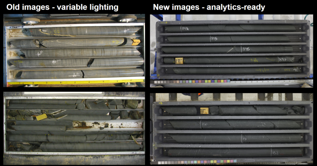
Figure 1: Examples of legacy core photos taken with variable lighting, vs those taken with an improved camera and lighting setup for analytics-ready images.

You’re surprised and confused when, despite the images being better, the model’s predictions seem to be worse. This is data drift: the distribution of the inputs (the pixels in the images) has changed. The model still knows how to do the task but it’s now encountering inputs it wasn’t trained on. It needs to be given examples of these higher-quality photographs and their labels in order to learn how to classify them well. The good news is with enough training data, the model should perform well across both the new analytics-ready photographs and the existing legacy images (Fig 2).

Another example of data drift in this context would be if the rocks themselves start changing – a sandstone becomes more silty, or you start drilling into a new lithology altogether.

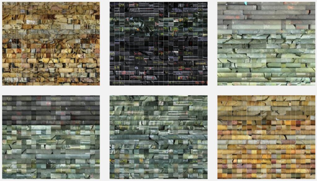
Figure 2: Core photos that have been chopped up into square tiles and classified based on lithology. Each panel shows tiles that have been predicted as a distinct lithology. The lower-left and upper-right panels show data drift due to different lighting conditions, which has been successfully handled by providing enough training data (the tiles are correctly classified despite the changed lighting).

Concept drift: When the same inputs mean something new

Concept drift is different. Here, the data doesn’t change, but the meaning of the data has changed. Often this can occur together with data drift, but let’s look at a couple of examples of ‘pure’ concept drift.

Scenario: Increasing Geological Resolution Over Time

At the start of a drilling program, your geology team classifies drillcore intervals into three lithologies: basalt, dolerite and sediment. They’re working quickly, logging hundreds of metres per day based on texture and colour. A machine learning model is trained on this early logging to automate lithological classification from images.

As more drilling is completed, the team realizes that the ‘dolerite’ includes at least two different intrusive phases: an early equigranular phase and a later porphyritic phase that correlates spatially with higher gold grades. 

They split their logging into early_dolerite and late_dolerite, and go back to relog some holes with the new classification. However, the model is still trained on the original, coarser classification scheme.

This is a classic example of concept drift. Given the same inputs (images of dark rocks with visible grains), the desired output has changed. In this example, it would be obvious to everyone that the model needs to be updated to classify the two dolerites separately.

But concept drift will not always be so obvious. Let’s consider another example where concept drift might occur without anyone noticing.

Scenario: Pathfinder Elements Lose Predictive Power

Your team builds a geochemical model to predict potential gold-bearing zones based on multielement assay data. During early drilling, the mineralization is clearly associated with elevated arsenic (As), antimony (Sb), and sericite alteration. You train a model to predict zones of likely gold mineralization using these patterns.

Over time, the drilling footprint expands. You start hitting gold in areas with lower As, more carbonate alteration, and no clear vectoring pattern from the original pathfinder elements.

The geochemistry looks within the range of previous samples – there is no data drift. But the relationship between those inputs and gold mineralization has changed. The model is still confidently flagging high-As zones as prospective, and missing low-As gold zones entirely.

Because the model outputs still “look reasonable” (e.g., it finds some mineralized holes), and no one has flagged a change in the alteration model (yet), it’s hard for your SME’s to notice that the model’s predictions have quietly degraded.

But eventually, they will keep seeing results that don’t make sense, and if nothing changes, your team’s trust in the model will be eroded.

Why drift matters

There are two significant consequences of unnoticed drift. The first, and most obvious, is that poor-quality model outputs will be used for decision-making, with all the operational consequences those decisions may have.

The second is more insidious – it can erode trust in machine learning systems generally. When SMEs notice that the model isn’t performing well, but don’t identify drift as the culprit, it would be easy to dismiss the whole idea of using machine learning for the task. This is a shame, because retraining the model could resolve the problem and allow the model to continue providing useful and timely information.

How to deal with drift

Details of drift detection are a subject for another day, but the basic idea is:

• Monitor incoming data over time – if new data is quite different to data used in model training, you may notice data drift
• Monitor model performance over time – ideally, continue providing small batches of validation data to check the model is still working well
• Keep SMEs in the loop – if something feels “off” to a geologist, investigate
• Retrain the model as needed, when drift is identified

A note on notation

To close things off, let’s explain drift using that mathematical notation.

• X = the input data that goes into the model. This could be things like geochemical assay results, the pixels in a drillcore photos, lithological logs, or geophysical data.
• y = the target or label the model is trying to predict. For example: gold mineralization (yes/no), rock type (basalt/dolerite/sediment), or grade estimates.
• P(X) = the probability distribution of the input data – in simple terms, how the values of X are spread out. If this changes over time, it’s called data drift.
• P(y|X) = the relationship between the inputs and the target.  This is what the model is trying to learn: “Given this input X, what’s the most likely y?”. If this changes over time, it’s concept drift. 

Think of X as the clues you give a detective, and y as the conclusion they draw.

• If the clues start looking different, that’s data drift.
• If the same clues now point to a different culprit, that’s concept drift.

Of course, in many cases, both types of drift will occur together – new clues, and new ideas about old clues.

Final thoughts

Drift is a natural consequence of working in real-world geological systems. Models trained on early data may not hold up as the project evolves. That doesn’t mean they’re not useful – they just need updating. Machine learning is never a set and forget exercise, models and systems need constant monitoring and validation to ensure they are always delivering the outcomes users expect and require.

The key is staying aware. By understanding how and why models fail, we can build workflows that adapt alongside our growing understanding of the geological problem.

References

Bayram, Firas, Bestoun S. Ahmed, and Andreas Kassler. “From Concept Drift to Model Degradation: An Overview on Performance-Aware Drift Detectors.” Knowledge-Based Systems 245 (June 2022): 108632. https://doi.org/10.1016/j.knosys.2022.108632.